Building GPT from Scratch: Following Karpathy’s Tutorial
The Transformer architecture has become the workhorse behind modern LLMs. GPT-2/3/4/5, Llama, Claude, Gemini: they all are built on top of the same core architecture or its variants from the 2017 “Attention Is All You Need” paper. I wanted to understand this architecture properly, so I followed Andrej Karpathy’s “Let’s Build GPT from Scratch” video. It’s a 2-hour walkthrough where you start from an empty file and end up with a working Transformer.
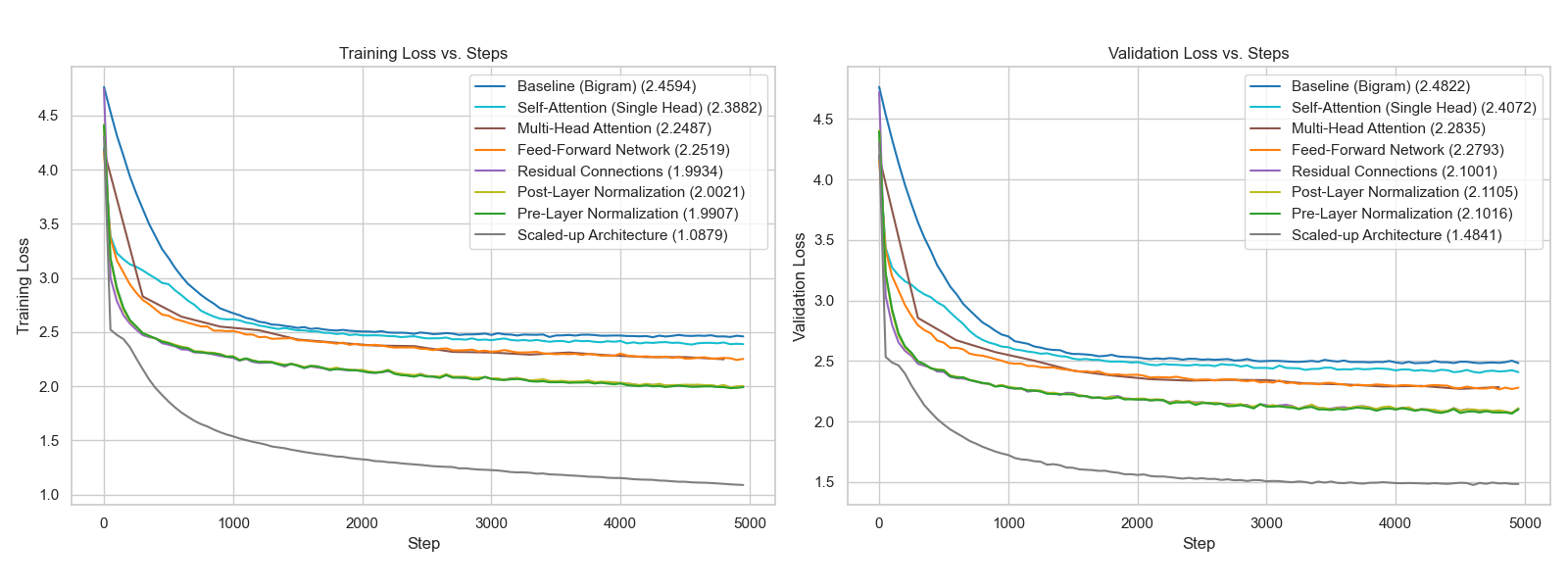
I followed Karpathy’s video and captured each architectural addition as a separate commit. This let me see exactly how each component pulled down the validation loss. In this walkthrough, the training data is ~1M characters of Shakespeare and the goal is to generate Shakespeare-like text.
| Component | Val Loss | Commit | |
|---|---|---|---|
| Baseline | Bigram Model | ~2.49 | e0b5864 |
| Update 1 | Single Head Self-Attention | ~2.4 | 7b0e03a |
| Update 2 | Multi-Head Attention | ~2.28 | 9d2a7b5 |
| Update 3 | Feed-Forward Network | ~2.27 | c4c46ff |
| Update 4 | Residual Connections | ~2.09 | 0239c07 |
| Update 5 | Layer Normalization | ~2.076 | 63ef5f8 |
| Update 6 | Pre-LayerNorm (modern) | ~2.076 | 4f5bef8 |
| Update 7 | Scaling Up + Dropout | ~1.48 | d4141d7 |
You can find all the code and notebooks in the repo: building-from-scratch/basic-gpt
Baseline: Bigram Model (e0b5864)
Karpathy starts with the simplest possible language model: a bigram model. It predicts the next character based only on the current character. No context at all. The tokens aren’t talking to each other.
This still works somewhat because some characters naturally follow others (the letter ‘q’ is almost always followed by ‘u’). But the output is complete gibberish because the model has no way to look at what came before.
Result: ~2.49 validation loss.
Update 1: Self-Attention (7b0e03a)
We want tokens to communicate with each other and predictions to consider context from previous tokens, not just the current one. A token at position 5 should be able to look at tokens 1-4 and gather information from them. But at the same time, it can’t look at tokens 6, 7, 8 because those are the future we’re trying to predict.
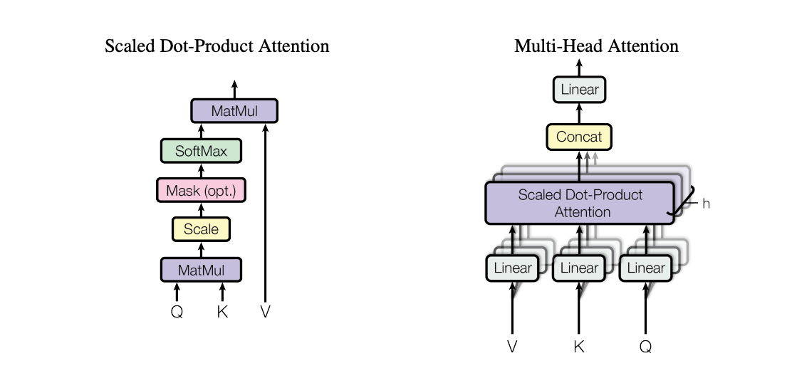
Self-attention solves this. Every token is represented by 3 vectors: - Query: “What am I looking for?” - Key: “What do I contain?”
- Value: “If you find me interesting, here’s what I’ll tell you.”
The query dot-products with all the keys. High dot product means high affinity: “I find you interesting.” The values of interesting tokens get aggregated via weighted sum.
Note: Attention is really a communication mechanism. You can think of it as nodes in a directed graph where every node aggregates information from nodes that point to it. In our case, token 5 can receive information from tokens 1-4 (and itself), but not from tokens 6-8. The triangular mask creates this directed structure and is what makes this a “decoder” block.
One subtle but important point: attention has no notion of space. The tokens don’t inherently know where they are in the sequence. That’s why we add positional embeddings. Each position gets its own learned embedding that’s added to the token embedding, giving the model spatial information.
Result: ~2.4 validation loss. Tokens can now see context.
Update 2: Multi-Head Attention (9d2a7b5)
Tokens have a lot to talk about. One head might look for consonants, another for vowels, another for word boundaries, another for patterns at specific positions. Having multiple independent communication channels lets the model gather diverse types of data in parallel.
Note: This is similar to grouped convolutions. Instead of one large convolution, you do it in groups. With 4 heads of 8 dimensions each, we get the same total dimensionality (32) but with 4 separate communication channels. Each head can specialize in different patterns.
Result: ~2.28 validation loss.
Update 3: Feed-Forward Network (c4c46ff)
The FFN layer addresses a key problem. Until now, “the tokens looked at each other but didn’t have enough time to think about what they found.”
Self-attention is the communication phase. Tokens gather data from each other. But then they need to compute on that data individually. That’s what the feed-forward network does. It operates on a per-token level. All the tokens process their gathered information independently.
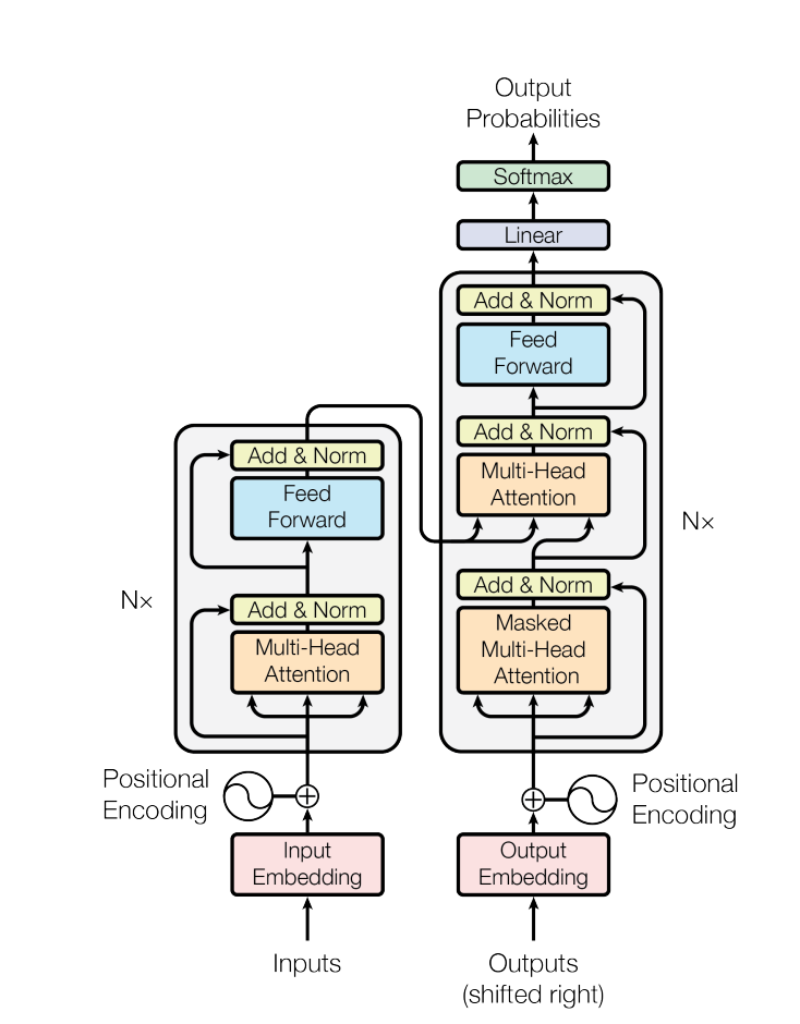
So the Transformer block becomes: communicate (attention) → compute (feed-forward). This pattern repeats for every layer.
Result: ~2.27 validation loss. The architecture now has both communication and computation.
Update 4: Residual Connections (0239c07)
This is one of two optimizations that make deep networks actually trainable. Without it, stacking many layers leads to vanishing gradients and optimization difficulties.
Karpathy visualizes it nicely: imagine a residual pathway running from top to bottom. You can “fork off” from this pathway, do some computation, and project back via addition. The path from inputs to outputs is just a series of additions.
Note: Why does this help? During backpropagation, addition distributes gradients equally to both branches. The gradients “hop” through every addition node directly to the input. This creates a “gradient superhighway” from supervision to input, unimpeded. The residual blocks are initialized to contribute very little at first, then “come online” over time during optimization.
Result: ~2.09 validation loss. Now we can stack layers without vanishing gradients.
Update 5 & 6: Layer Normalization (63ef5f8, 4f5bef8)
Batch normalization normalizes columns (across examples in a batch). Layer normalization normalizes rows (across features for each example). The implementation is almost identical, you just change which dimension you normalize over.
Layer norm has advantages for Transformers: - No dependency on batch size (works even with batch size 1) - No running buffers to maintain - No distinction between training and test time
The original Transformer paper used post-layer norm (normalize after attention/FFN). Modern implementations use pre-layer norm (normalize before). Pre-layer norm creates a cleaner residual pathway since the transformation happens on normalized inputs, leading to more stable training.
Result: ~2.076 validation loss.
Update 7: Scaling Up (d4141d7)
With all the architectural pieces in place, Karpathy scales up the architecture:
| Parameter | Before | After |
|---|---|---|
| Block size (context) | 8 | 256 |
| Embedding dim | 32 | 384 |
| Heads | 4 | 6 |
| Layers | 3 | 6 |
| Dropout | 0 | 0.2 |
Dropout is added for regularization. It randomly shuts off neurons during training, effectively training an ensemble of sub-networks. At test time, everything is enabled and the sub-networks merge.
Result: ~1.48 validation loss. The generated text now looks like Shakespeare (structure, dialogue formatting, character names) even though it’s nonsensical when you actually read it.
How This Compares to GPT-3
| My Model | GPT-3 | |
|---|---|---|
| Parameters | ~10M | 175B |
| Dataset | ~300K tokens | 300B tokens |
| Architecture | Nearly identical | Nearly identical |
The architecture we built is essentially the same as GPT-3. The difference is pure scale: 17,500x more parameters trained on 1 million times more data. By today’s standards, even GPT-3’s 300B tokens is considered modest. Current models train on 1T+ tokens.
This is what makes the Transformer architecture so remarkable. The same fundamental design (attention for communication, feed-forward for computation, residual connections, layer norm) scales from a 10M parameter Shakespeare generator to a 175B parameter model!
Resources
- Code: building-from-scratch/basic-gpt
- Video: Let’s Build GPT from Scratch by Andrej Karpathy